|
Objective:
The learner will understand,
through a hands-on experience, the
basic concepts behind the use and working of a laser altimeter
for the study of solar system topography.
Outcomes:
- Students will plot and graph data they have collected using a
hands-on version of laser altimetry.
- Students will gain an understanding of the use of laser altimetry
in the study of planetary topography.
Introduction:
January 10, 1999, the satellite NEAR begins an orbit of 433 Eros, which makes it the first spacecraft to orbit, and study, an asteroid. One of the instruments aboard the satellite is a laser altimeter. The laser will be used to take topographical measurements of the surface of 433 Eros. With this data, topographical maps and 3 dimensional models will be created. This activity will introduce you to the concept of laser altimetry and how the data is used in order to create maps and model solar system bodies.
Materials:
Ping-pong ball
wooden blocks of various sizes
masking tape - 2 pieces @ 10 cm each (optional)
meter stick
stop watch
graph paper (enough for 3 graphs per group)
pen/pencil
Procedure:
This activity requires
at least two people per group. Three people
per group would be the optimum. The jobs can be rotated if group
members so desire. Read through the whole activity before beginning.
STEP ONE:
- Choose a spot on a wall 2.2 m or higher from the floor, and place
one 10 cm length of tape on the wall, at that height, parallel
to the floor. (You may need a chair.)
- Holding the ball next to the tape on the wall, between your first
finger and thumb, drop it and watch to see how high it bounces
back up. Mark that spot on the wall with your finger. It is best
to do this step two or three times to determine the highest point
of return. (Using the mortar lines on cinder block walls will
work well, too. Be sure to use the same two lines throughout this
whole activity.)
- Measure 45 cm toward the floor and mark this spot with the second
piece of tape. This will be the constant for measuring the time
for the ping-pong ball's period.
- Measure the distance from the first piece of tape (or mortar line)
to the floor and back up to the second tape line. Record this
on your data sheet. This distance will be used to create a baseline
for all other measurements, so be as precise as you can.
- As in number two, one partner should hold the ping-pong ball next
to the higher piece of tape, between the first finger and thumb,
and approximately one inch from the wall.
- One partner should have a stopwatch and have his/her eyes level
with the second piece of tape. A third partner, if available should
be recording the results of each ball drop using the attached
data sheet or one that your group makes up for itself. * Note: A
spreadsheet would work well for recording and calculating
this data.
- Drop the ball, and as you do say, "Go." The timer starts
the stopwatch
on "Go."
- The timer will stop the watch when the ball rebounds and reaches
the lower line. (His/her eyes should be level with the lower piece
of tape. The time should be stopped as soon as any part of the
ball touches any part of the line.) Record the time on the data
sheet. Repeat this step four more times.
- Calculate the velocities (V=D/T). After finding the velocity for
each of the trials, find the average velocity of the ping-pong
ball. This average will be used later in this lab. It will be
your baseline for comparing data.
STEP TWO:
Now that you have found the
velocity of the ping-pong ball, you
will use this information to plot the topography along a line
of latitude of an asteroid. You will be creating your own asteroid
terrain on the floor against the wall where you just did Step
One.
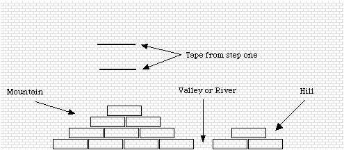
- Create the topography model of your asteroid, along the wall
where you did Step One. In order to
do this you need to place the wooden blocks against the wall in
a line about 6-8 feet long. Be sure that you build
in some hills, mountains, valleys, etc. (See Figure A)
- If you used tape in Step One instead of the mortar lines, you
will probably want to add new lengths of tape to the originals
that extend over the entire length of your topographical model.
Be sure that the new lines remain parallel to the floor so that
the heights don't change along the length of the model.
- Starting at the beginning of the top piece of tape, place a mark
every 20cm. The bottom piece does not need to be marked.
- Again, starting at first interval mark you made at the beginning
of the tape, you will drop the ping-pong ball as you did in Step
One, and record the time in Data Table II. Drop the ball and record
the results two more times. Be sure to be as accurate as you can
with the timing.
- Repeat number four for each of the interval marks you placed on
the wall.
- Find the average time for each of the intervals and record it
on the data table.
STEP THREE: PLOTTING AND GRAPHING THE DATA:
You will now plot the data for
the average times and create graphs
of the altimetry readings for your topographic model. The graphs
will use different intervals between readings, so that you can
compare the preciseness of different levels of accuracy (called
spatial resolution).
- Graph 1
- Plot the average time for every 60cm interval. (0cm, 60cm, 120cm,
etc.)
- Connect the points with a smooth line.
- Label the graph appropriately.
- Graph 2
- Plot the average time for every 40cm interval.
- Connect the points with a smooth line.
- Label the graph appropriately.
- Graph 3
- Plot the average time for every 20cm interval.
- Connect the points with a smooth line.
- Label the graph appropriately.
PING-PONG ALTIMETER
Data Table I
| Drop |
Distance ball traveled |
Time (seconds) |
Velocity (distance/time) |
| 1 |
|
|
|
| 2 |
|
|
|
| 3 |
|
|
|
| 4 |
|
|
|
| 5 |
|
|
|
|
|
Average Velocity |
________________
|
PING-PONG ALTIMETER
Data Table II
| Interval |
Trial 1 |
Trial 2 |
Trial 3 |
Average Time (sec) |
Distance Ball Traveled (cm) |
| 0cm |
|
|
|
|
|
| 20cm |
|
|
|
|
|
| 40cm |
|
|
|
|
|
| 60cm |
|
|
|
|
|
| 80cm |
|
|
|
|
|
| 100cm |
|
|
|
|
|
| 120cm |
|
|
|
|
|
| 140cm |
|
|
|
|
|
| 160cm |
|
|
|
|
|
| 180cm |
|
|
|
|
|
| 200cm |
|
|
|
|
|
| 220cm |
|
|
|
|
|
| 240cm |
|
|
|
|
|
| 260cm |
|
|
|
|
|
| 280cm |
|
|
|
|
|
| 300cm |
|
|
|
|
|
PING-PONG ALTIMETER
Data Table III
|
°R
Interval |
Original Distance Ball Traveled (From Data Table
One) {D1} |
Distance Ball Traveled (cm) {D2} |
Altitude (cm) {D1-D2= Altitude} |
| 0cm |
|
|
|
| 20cm |
|
|
|
| 40cm |
|
|
|
| 60cm |
|
|
|
| 80cm |
|
|
|
| 100cm |
|
|
|
| 120cm |
|
|
|
| 140cm |
|
|
|
| 160cm |
|
|
|
| 180cm |
|
|
|
| 200cm |
|
|
|
| 220cm |
|
|
|
| 240cm |
|
|
|
| 260cm |
|
|
|
| 280cm |
|
|
|
| 300cm |
|
|
|
Use your graphs and data to answer the remaining
questions
- Why is it important to keep the distance between each altimeter measurement consistent?
- How could we make the topographical profile more accurate?
- What does the graph look like in comparison to your model (i.e.. the same, inverted, etc.)?
- Which looks more like the model, the graph you generated from the shorter or longer distances between readings (intervals)?
- What will you have to do to the data to make the graph look right-side up?
The
Laser Rangefinder aboard NEAR sends out a laser beam and
“catches”
it as it returns from being reflected by the surface of 433 Eros.
The instrument records how long it takes the beam to reach the
surface and bounce back up. The scientists know how fast the beam
is traveling; therefore, they can calculate how far it traveled. By
measuring this time and multiplying by the velocity
of the beam, they calculate how far the laser has traveled. They
must then divide the distance the beam traveled in half.
Why did you not divide in half to find the distance to the object
in your topography model?
Next, the scientist must compare
this distance to a "baseline"
distance we will call zero. On Earth, we might use sea level as
the baseline. Another way to set the baselines is to start at
the center of the planetary body being studied and draw a perfect
circle as close to the surface of the body as possible. Using
this baseline, the altitude compared to zero can be calculated
and graphed. (Here, on Earth, we often say that some point is
a certain number of feet above of below sea level.)
Why do we not use the term "Sea level" for Mars and other
planets?
You will now calculate the altitude of the points along your model.
To do this subtract the distance the ball traveled, at each interval
(from Data Table II) from the distance the ball traveled in Step
One (column B, Data Table I). The number you come up with will
be zero or greater. Use Data Table III to do your calculations.
{The number in column B in this table should be the same for every
interval. Remember, it was the baseline altitude and does not
change.}
|